Initialization
In the following, we will discuss how to initialise the various models from a common set of initial data, namely
- the guiding center position $X$ in physical coordinates,
- the particle energy $W$ in eV,
- the particle mass $m$ in kg,
- the particle charge number,
- the gyro angle $\theta \in [0, 2\pi]$,
- the pitch angle $\alpha \in [0, \pi / 2]$.
For charged particles we need to convert the energy into a velocity vector. For the Pauli particle we need to compute the coordinates of the guiding centre $X$ of the particle and construct a velocity vector that only holds the component of the velocity that is parallel to the magnetic field, while the perpendicular component goes into the magnetic moment $\mu$. For the guiding center, we need the same coordinate transformation as for the Pauli particle, but we only need the absolute value of the velocity in direction of the magnetic field $u$ and the magnetic moment $\mu$.
Make sure to read about the Normalization before proceeding.
Velocities
Set $e = e' \hat{e}$ with $e' = 1.602 176 634 \cdot 10^{-19}$ and $\hat{e} = \mathrm{C}$ and similarly $m = m' \hat{m}$ with $\hat{m} = \mathrm{kg}$. Some common values for the mass are
| Particle | Normalised Mass $m'$ |
|---|---|
| electron | $9.1093837015 \cdot 10^{-31}$ |
| proton | $1.6726219237 \cdot 10^{-27}$ |
| deuteron | $3.3435837724 \cdot 10^{-27}$ |
| alpha | $6.6446573357 \cdot 10^{-27}$ |
The absolute value of the velocity is obtained from the particle energy by $\vert v \vert^2 = 2 W / m$. In normalised units, we have $W = W' \hat{W}$ and $v = v' \hat{v}$ where $\hat{W} = e \mathrm{V}$ and $\hat{v} = \hat{l} \hat{\omega}_c = \hat{l} \hat{B} e / m$.
Let us compute the normalised kinetic energy,
\[\frac{\vert v' \vert^2}{2} = \frac{W' \hat{W}}{m \hat{v}^2} = \frac{W' e \mathrm{V} m^2}{m \hat{l}^2 \hat{B}^2 e^2} .\]
Usually, we have $\hat{B} = T = \mathrm{kg} / \mathrm{C}\,\mathrm{s}$. Recall that $\mathrm{V} = \mathrm{kg}\,\mathrm{m}^2 / \mathrm{C}\,\mathrm{s}^2$ and let us set $\hat{l} = l_0 \mathrm{m}$, then
\[\frac{\vert v' \vert^2}{2} = \frac{m' W'}{e' l_0^2} .\]
Thus for the absolute value of the velocity we have
\[\vert v' \vert = \frac{1}{l_0} \sqrt{ 2 W' \, \frac{m'}{e'} } .\]
The pitch angle $\alpha$ determines the distribution of the kinetic energy into the perpendicular and parallel components by
\[\begin{aligned} W_{\perp}' &= W' \sin \alpha , \qquad W_{\parallel}' &= W' \, (1 - \sin \alpha) . \end{aligned}\]
Note that this is not the textbook pitch-angle convention $W_{\perp} = W \sin^{2} \alpha$, $W_{\parallel} = W \cos^{2} \alpha$; it is however self-consistent with the inverse relation $\alpha = \arcsin (W_{\perp}' / W')$ used by InitialConditionsGC to recover the pitch angle from $(u, \mu)$. and accordingly
\[\begin{aligned} \vert v_{\perp}' \vert &= \frac{1}{l_0} \sqrt{ 2 W_{\perp}' \, \frac{m'}{e'} } , \qquad \vert v_{\parallel}' \vert &= \frac{1}{l_0} \sqrt{ 2 W_{\parallel}' \, \frac{m'}{e'} } . \end{aligned}\]
For each equilibrium, the ElectromagneticFields.jl package generates an orthonormal triad $(a, b, c)$, where $b$ is the unit vector of the magnetic field and $a$ and $c$ span the plane perpendicular to it. The triad is exposed in three different component representations, which coincide only in Cartesian coordinates:
| Functions | Components |
|---|---|
a♭(field,t,x), b♭(field,t,x), c♭(field,t,x) | covariant |
a♮(field,t,x), b♮(field,t,x), c♮(field,t,x) | physical |
a♯(field,t,x), b♯(field,t,x), c♯(field,t,x) | contravariant |
The velocity vector $v$ is assembled in physical coordinates, that is from a♮, b♮ and c♮, and subsequently transformed to contravariant coordinates with the inverse Jacobian DF̄. The function b♮ returns the unit vector of the magnetic field, thus
\[v_{\parallel}' = \vert v' \vert \, \sqrt{1 - \sin \alpha} \, b .\]
The functions a♮ and c♮ return two unit vectors that span the plane perpendicular to the magnetic field, thus
\[v_{\perp}' = \vert v' \vert \, \sqrt{\sin \alpha} \, ( - a \, \sin \theta - c \, \cos \theta ) ,\]
where $\theta$ is the gyro angle. The magnetic moment is computed as
\[\mu = \frac{ \vert v_{\perp}' \vert^2 }{2 \vert B' \vert} = \frac{ \vert v' \vert^2 \sin \alpha }{2 \vert B' \vert} .\]
Gyro-radius Vector and Position
In order to compute the particle position, we need to construct the gyro radius vector $\rho$, which is given by
\[\rho = \frac{b \times v}{\omega_c} = \frac{b \times \hat{v} v'}{\hat{\omega}_c \omega_c'} = \hat{l} \, \frac{b \times v'}{\vert B' \vert} .\]
Here we used $\hat{v} / \hat{\omega}_c = \hat{l}$, which follows from $\hat{v} = \hat{l} \hat{\omega}_c$, and recall that $\hat{l} = l_0 \mathrm{m}$. Note that
\[\omega_c = \frac{e \vert B \vert}{m} = \frac{e \vert \hat{B} B' \vert}{m} = \frac{e \vert \hat{B} \vert}{m} \vert B' \vert = \hat{\omega}_c \omega_c' ,\]
as
\[\hat{\omega}_c = \frac{e \vert \hat{B} \vert}{m} ,\]
so that
\[\omega_c' = \vert B' \vert .\]
The normalized gyro radius vector reads
\[\rho' = \frac{\rho}{\hat{l}} = \frac{b \times v'}{\vert B' \vert} ,\]
so that the normalised particle position is
\[x' = X' + \rho' .\]
The gyro phase $\theta$ is defined as the angle, measured in the clockwise sense, between $a$ and $\rho$, so that
\[\frac{b \times v'}{\vert v' \vert \, \sin \alpha} = a \, \cos \theta - c \, \sin \theta .\]
Guiding Center Coordinates
Instead of the particle energy $W$ and pitch angle $\alpha$, we can also compute all initial conditions from the guiding center initial data, i.e., parallel velocity $u = \vert v_{\parallel} \vert$, magnetic moment $\mu$ and gyro angle $\theta$.
Start by computing the absolute value of the perpendicular velocity by
\[\vert v_\perp \vert = \sqrt{ 2 \mu \vert B \vert } ,\]
and the total velocity by
\[\vert v \vert = \sqrt{ \vert v_{\parallel} \vert^2 + \vert v_\perp \vert^2 } .\]
With that, we can compute the perpendicular and total energy,
\[\begin{aligned} W_{\perp}' &= \frac{e l_0^2 \vert v_\perp \vert^2}{2m} , \qquad W' &= \frac{e l_0^2 \vert v \vert^2}{2m} . \end{aligned}\]
The pitch angle is obtained as
\[\alpha = \arcsin \frac{W_{\perp}'}{W'} .\]
With that, the rest of the quantities can be computed in the same way as above.
Initial Conditions
ChargedParticleDynamics.jl provides the InitialConditions module for the computation of the above quantities. Three functions are provided that return the initial conditions for the different models. For charged particles the initial conditions are $(x', v')$, for the Pauli particle we have $(X', v_{\parallel}', \mu)$ and for the guiding center we use $(X', u', \mu)$ with $u' = \vert v_{\parallel}' \vert$.
Everything on this page describes machinery that is available but not wired up. Each equilibrium module carries its u and μ as hard-coded literals rather than deriving them from a position, a pitch angle and an energy through InitialConditions. The only callers of these functions are this page, the ITER Equilibrium in Cylindrical Coordinates example and scripts/guiding_center_3d.jl.
The literals are also not reproducible from the functions here. For the small tokamak in cartesian coordinates, whose Pauli module declares xᵢ = [1.05, 0, 0] and vᵢ = [2.1e-3, 4.3e-4, 0], the parallel velocity $v \cdot b$ comes out at 0.00042987 against a hard-coded 0.00045136, and $\vert v_{\perp} \vert^{2} / 2B$ at 2.31459e-6 against a hard-coded 2.310e-6 — the latter being a nearby but different number rather than the same one rounded. Where the shipped values came from is not recorded anywhere in the repository, so the per-equilibrium docstrings say so rather than inventing a derivation.
Routing the equilibrium modules through this layer is the fix, and is the task One initial-conditions layer for all models in TODO.md. It would make u and μ derived quantities that a new equilibrium gets for free, at the cost of shifting the shipped values by the percentages above.
ChargedParticleDynamics.InitialConditions — Type
Store initial conditions for charged particle, Pauli particle and guiding center models.
Fields:
x: particle positionX: gyro center positionρ: gyro radius vectorvvec: velocity vectorvpar: parallel velocity vectorvper: perpendicular velocity vectorv: absolute value of velocityu: absolute value of parallel velocityμ: magnetic momentθ: gyro angle ∈ [0,2π]α: pitch angle ∈ [0,π/2]ω: gyro frequencymass: mass in kgenergy: energy in eVcharge: charge number
ChargedParticleDynamics.InitialConditions — Method
InitialConditions(X, θ, α, E, M, C, field; l₀ = 1)
InitialConditionsGC(X, θ, u, μ, M, C, field; l₀ = 1)
The same, with the eight field functions read from field, an ElectromagneticFields field.
ChargedParticleDynamics.InitialConditions — Method
Compute initial conditions from the following arguments:
X: gyro center positionθ: gyro angleα: pitch angleE: energyM: massC: charge numberâ,b̂,ĉ: magnetic field unit vectors in physical coordinates (a♮,b♮,c♮)b: magnetic field unit vector in contravariant coordinates (b♯)B: amplitude of magnetic fieldg̅: inverse metric coefficients (g♯)DF̄: inverse Jacobian matrixJ: Jacobian determinantl₀ = 1: length normalization
ChargedParticleDynamics.InitialConditionsGC — Method
Compute initial conditions from the following arguments:
X: gyro center positionθ: gyro angleu: absolute value of parallel velocityμ: magnetic momentM: massC: charge numberâ,b̂,ĉ: magnetic field unit vectors in physical coordinates (a♮,b♮,c♮)b: magnetic field unit vector in contravariant coordinates (b♯)B: amplitude of magnetic fieldg̅: inverse metric coefficients (g♯)DF̄: inverse Jacobian matrixJ: Jacobian determinantl₀ = 1: length normalization
ChargedParticleDynamics.cartesian_solution — Method
cartesian_solution(sol)
cartesian_solution(sol, field)
The solution sol in cartesian coordinates, together with the major radius: a named tuple of the time series and the R, X, Y and Z data series. The coordinate helpers come from coordinates(field), so the field must be axisymmetric; the one-argument form takes it from the solution's own parameters.
ChargedParticleDynamics.charged_particle — Method
Extracts the charged particle initial conditions and returns the tuple (x,v). If the keyword argument noncanonical is set to true, the functions returns the vector vcat(x,v).
ChargedParticleDynamics.check_chart — Method
check_chart(field, reference)Throw an ArgumentError unless field holds an equilibrium of the same kind as reference, and so one written in the same chart. A formula that an equilibrium module writes in its own coordinates — its toroidal_momentum, which is ϑ₃ where the third coordinate is the toroidal angle and x ϑ₂ - y ϑ₁ in a cartesian chart — is right only for a field in that chart, while the right-hand sides take a field in any orthogonal chart.
ChargedParticleDynamics.guiding_center — Method
Extracts the guiding center initial conditions and returns the tuple (vcat(X,u),μ).
ChargedParticleDynamics.pauli_particle — Method
Extracts the Pauli particle initial conditions and returns the tuple (X,vpar,μ). If the keyword argument noncanonical is set to true, the functions returns the tuple (vcat(X,vpar),μ).
ChargedParticleDynamics.periodic_domain — Method
periodic_domain(field, T, n)The periodic domain of an n-component state whose first three components are the coordinates of field's chart, as the (xmin, xmax) tuple that GeometricEquations takes as periodicity.
A component is periodic where periodic(field) says so, and wraps on the chart's own rangemin/rangemax. Every other component, including every one past the third, gets $(-\infty, +\infty)$.
periodic(field) answers one Bool per coordinate and is not itself a periodicity: passed in its place, a three-element vector destructures to (false, false) without any error. A bounded range does not imply periodicity either, which is why the bounds are taken only where periodic says so.
Example
As an example, let us consider a deuteron in an ITER-like analytical equilibrium (obtained from ElectromagneticFields.SolovevEquilibriumITER). The guiding center position is $[7, 0, 0]$, the energy is $1 \, \mathrm{MeV}$, and the pitch angle is $\pi / 2$.
| Fields | Value |
|---|---|
x | [1.129032258064516, -0.005902625716371616, 1.1084431084484293e-5] |
X | [1.129032258064516, 0.0, 0.0] |
ρ | [-3.5276395759963886e-21, -0.005902625716371616, 1.1084431084484293e-5] |
v⃗ | [-0.0044691509891760005, 6.0983271833801295e-6, 0.0025475918926682523] |
v∥ | [0.0, 6.0983271833801295e-6, 0.0025475918926682523] |
v⟂ | [-0.0044691509891760005, 0.0, 0.0] |
v | 0.032951426156967195 |
u | 0.017833183330406035 |
μ | 0.0005070194648182152 |
θ | 0.0 |
α | 0.7853981633974483 |
ω | 3.628081135085401e7 |
M | 3.3435837724e-27 |
E | 1.0e6 |
C | 1 |
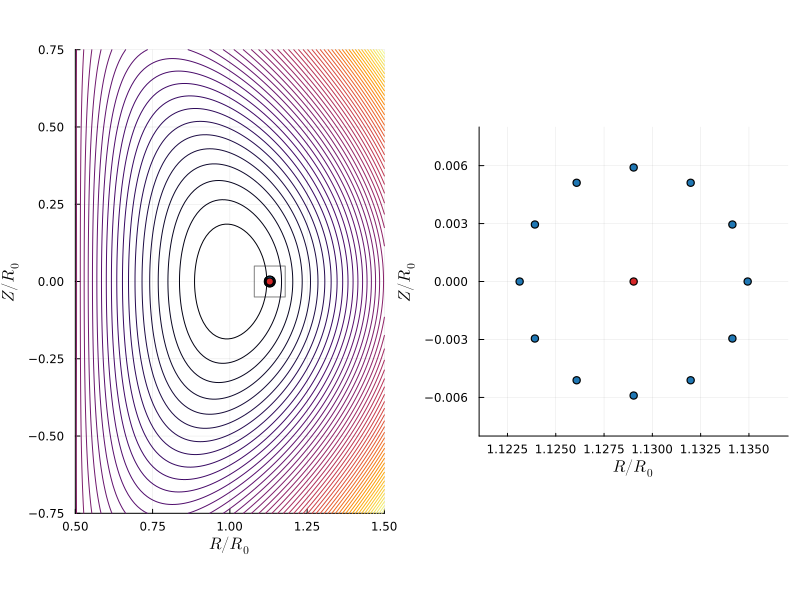
Below we plot the guiding center position (in red) and the particle position (in blue) in the poloidal plane for various gyro angles $\in [0, 2\pi]$. The right panel zooms into the white box around the guiding center.