Arnold-Beltrami-Childress Field
ElectromagneticFields.ABCEquilibrium — Type
Arnold-Beltrami-Childress (ABC) field in (x,y,z) coordinates with covariant components of the vector potential given by
\[A (x,y,z) = \big( a \, \sin(z) + c \, \cos(y) , \, b \, \sin(x) + a \, \cos(z) , \, c \, \sin(y) + b \, \cos(x) \big)^T\]
resulting in the magnetic field $B(x,y,z) = A(x,y,z)$.
Parameters: a, b, c
Constructing the Field
The three parameters a, b and c all default to one. If one of them vanishes the field lines are integrable, the flow reducing to a two-dimensional one. When all three are non-zero, regions of chaotic field lines appear alongside regular ones — including for $a = b = c$, the case in which they were first studied (Dombre et al., 1986).
using CairoMakie
using ElectromagneticFields

equ = ABCEquilibrium(1.0, 0.5, 0.5)
ABC Equilibrium with
A = 1.0
B = 0.5
C = 0.5Plotting
Since the ABC field is genuinely three-dimensional, the plot shows the absolute value of the magnetic field in the three mid-planes $z = \pi$, $y = \pi$ and $x = \pi$:
plot_equilibrium(equ)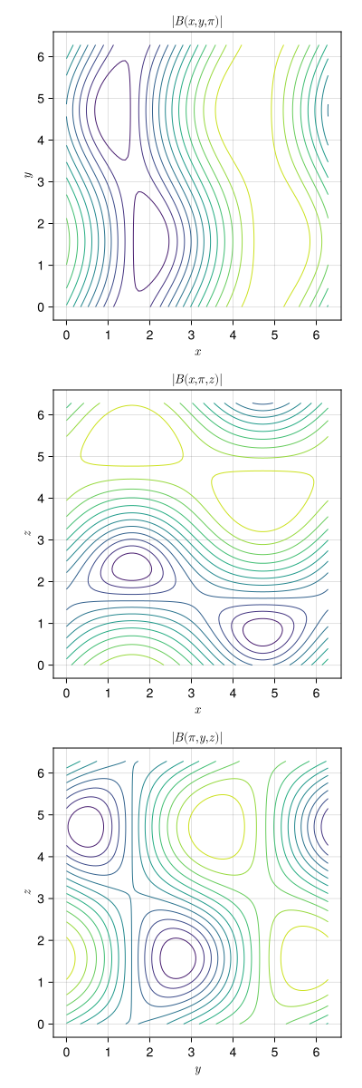
Evaluating the Field
field = FieldFunctions(ABCEquilibrium(1.0, 0.5, 0.5))Because $B = A$ for this field, the vector potential is the more interesting quantity to look at. Here it is sampled on a three-dimensional grid over one period:
nx, ny, nz = 100, 110, 120

xgrid = LinRange(0, 2π, nx)
ygrid = LinRange(0, 2π, ny)
zgrid = LinRange(0, 2π, nz)

potential(c) = [A♭(field, 0.0, xgrid[i], ygrid[j], zgrid[k])[c]
                for i in eachindex(xgrid), j in eachindex(ygrid), k in eachindex(zgrid)]

A_x = potential(1)
A_y = potential(2)
A_z = potential(3)

size(A_x)
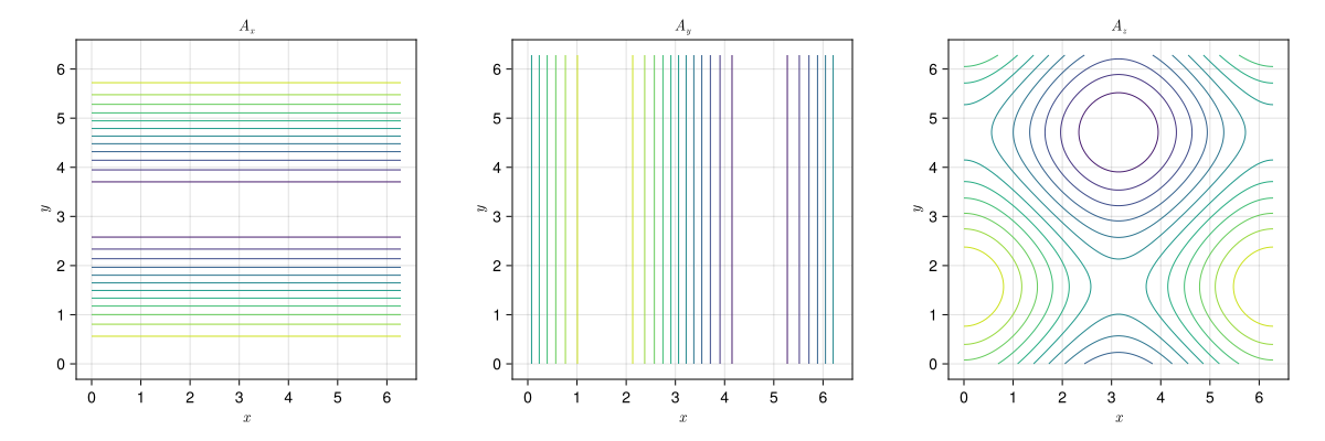
(100, 110, 120)Cutting through the middle of the $z$ range gives the three components in the $(x,y)$ plane:
k = div(nz, 2)

fig = Figure(size = (1200, 400))

for (n, (vals, label)) in enumerate(((A_x, L"A_x"), (A_y, L"A_y"), (A_z, L"A_z")))
    ax = Axis(fig[1,n]; xlabel = L"x", ylabel = L"y", title = label, aspect = DataAspect())
    contour!(ax, xgrid, ygrid, vals[:,:,k]; levels = 12)
end

fig