Quadratic Potentials

ElectromagneticFields.QuadraticPotentials — Module

Electromagnetic field with quadratic potentials in (x,y,z) coordinates Based on Xinjie Li, Ruili Zhang, and Jian Liu, Symplectic Runge-Kutta methods for the guiding center dynamics.

The covariant components of the vector potential are given by

\[A (x,y,z) = \bigg( -50y , \, 50x , \, \frac{x^2 + y^2}{2} \bigg)^T ,\]

resulting in the magnetic field with covariant components

\[B (x,y,z) = \big( y, \, -x, \, 100 \big)^T ,\]

and electrostatic potential

\[\phi (x,y,z) = \frac{1}{2} \big( x^2 + y^2 + z^2 \big) .\]

source

Constructing the Field

using CairoMakie
using ElectromagneticFields

equ = QuadraticPotentials.init()

Electromagnetic field with quadratic potentials in (x,y,z) coordinates

Plotting

The three components of the vector potential in the plane $z = 0$. The first two are linear in the coordinates, the third is quadratic:

plot_equilibrium(equ)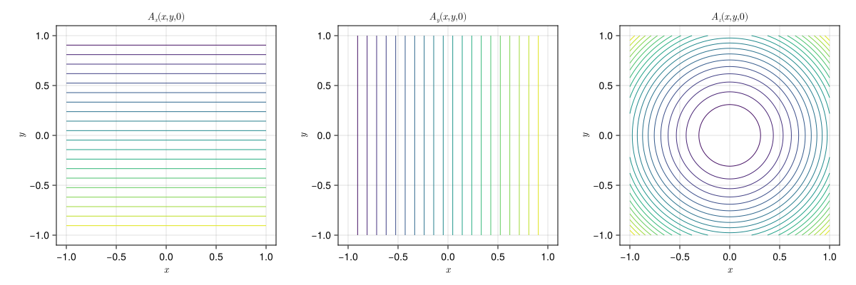

Evaluating the Field

This is one of the few fields that carries an electrostatic potential as well as a magnetic one, so the generated code includes φ and the components of the electric field:

QuadraticPotentials.@code()

t = 0.0
x = [0.5, 0.3, 0.2]

φ(t, x), [E₁(t, x), E₂(t, x), E₃(t, x)]

(0.19, [-0.5, -0.3, -0.2])