Axisymmetric Tokamak (Cartesian)
ElectromagneticFields.AxisymmetricTokamakCartesianEquilibrium — Type
Axisymmetric tokamak equilibrium in (x,y,z) coordinates with covariant components of the vector potential given by
\[A (x,y,z) = \frac{1}{2} \frac{B_0}{q_0} \, \bigg( \frac{q_0 R_0 x z - r^2 y}{R^2} , \, \frac{q_0 R_0 y z + r^2 x}{R^2} , \, - q_0 R_0 \, \ln \bigg( \frac{R}{R_0} \bigg) \bigg)^T ,\]
resulting in the magnetic field with covariant components
\[B (x,y,z) = \frac{B_0}{q_0} \, \bigg( - \frac{q_0 R_0 y + x z}{R^2} , \, \frac{q_0 R_0 x - y z}{R^2} , \, \frac{R - R_0}{R} \bigg)^T ,\]
where $R = \sqrt{ x^2 + y^2 }$ and $r = \sqrt{ (R - R_0)^2 + z^2 }$.
Parameters:
R₀: position of magnetic axisB₀: B-field at magnetic axisq₀: safety factor at magnetic axis
AxisymmetricTokamakCartesianITER returns this equilibrium with ITER's parameters.
Constructing the Field
using CairoMakie
using ElectromagneticFields

equ = AxisymmetricTokamakCartesianEquilibrium()
Axisymmetric Tokamak Equilibrium in (x,y,z) Coordinates with
R₀ = 1
B₀ = 1
q₀ = 2Plotting
The flux surfaces of this equilibrium are circular. In the $(x,z)$ plane at $y = 0$ the $y$ component of the vector potential is the physical toroidal component $A_\phi$, so $R \, A_y$ is the poloidal flux function and its contours are the flux surfaces:
plot_equilibrium(equ)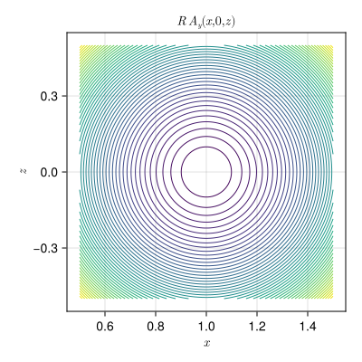
The same field in cylindrical and toroidal coordinates is available as well, which makes this a convenient test case for coordinate transformations.