Symmetric Solov'ev Equilibrium
ElectromagneticFields.SolovevSymmetricEquilibrium — Type
Symmetric Solov'ev equilibrium in cartesian (x,y,z) coordinates. Based on McCarthy, Physics of Plasmas 6, 3554, 1999.
The covariant components of the vector potential are given by
\[A (x, y) = \frac{B_0}{2} \, \bigg( 0 , \, 0 , \, - \frac{\alpha}{4} (R_0 + x)^4 - \beta y^2 \bigg)^T ,\]
Parameters:
R₀: major radius, which places the magnetic axis atx = -R₀B₀: B-field at magnetic axisα,β: free constants
Constructing the Field
The parameters are the major radius $R_0$, the field strength $B_0$, and the two coefficients $\alpha$ and $\beta$ of the flux function. The flux function depends on $x$ through $(R_0 + x)^4$, so $R_0$ shifts the magnetic axis to $x = -R_0$; taking $R_0 = 0$ puts it at the origin:
using CairoMakie
using ElectromagneticFields

equ = SolovevSymmetricEquilibrium(0.0, 1.0, 2.0, 0.5)
Quadratic Solovev Equilibrium with
R₀ = 0.0
B₀ = 1.0
α = 2.0
β = 0.5Plotting
Unlike the general Solov'ev equilibrium, this one is written in cartesian coordinates. Its flux surfaces are the contours of $A_z$, and because the flux function involves $x$ and $y$ only as $(R_0 + x)^4$ and $y^2$, they are symmetric both up/down and left/right about the magnetic axis:
plot_equilibrium(equ)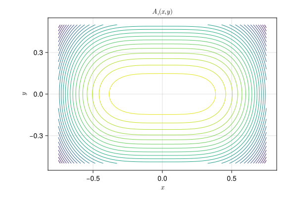
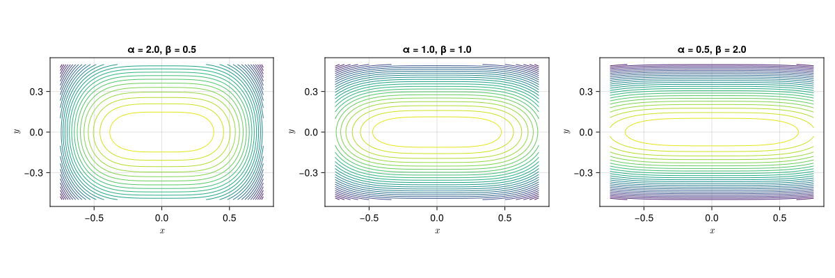
$\alpha$ weights the quartic dependence on $x$, $\beta$ the quadratic one on $y$, so it is their ratio that decides the shape of the surfaces — the larger $\beta / \alpha$, the flatter they get:
fig = Figure(size = (1200, 400))

for (n, (α, β)) in enumerate(((2.0, 0.5), (1.0, 1.0), (0.5, 2.0)))
    plot_equilibrium!(fig[1,n], SolovevSymmetricEquilibrium(0.0, 1.0, α, β);
        title = "α = $α, β = $β")
end

fig