Singular Field
ElectromagneticFields.SingularEquilibrium — Type
Singular magnetic field in (x,y,z) coordinates with covariant components of the vector potential given by
\[A (x,y,z) = \frac{B_0}{\sqrt{(x^2 + y^2)}^3} \big( y , \, - x , \, 0 \big)^T\]
resulting in the magnetic field with covariant components
\[B(x,y,z) = B_0 \, \begin{pmatrix} 0 \\ 0 \\ (x^2 + y^2)^{-3/2} \\ \end{pmatrix}\]
Parameters: B₀
Constructing the Field
using CairoMakie
using ElectromagneticFields

equ = SingularEquilibrium()
Singular Magnetic FieldPlotting
Both the vector potential and the magnetic field diverge as the $z$ axis is approached — the potential like $r^{-2}$, the field like $r^{-3}$ — so linearly spaced contour levels would show nothing but the singularity. The plot therefore uses logarithmically spaced levels:
plot_equilibrium(equ)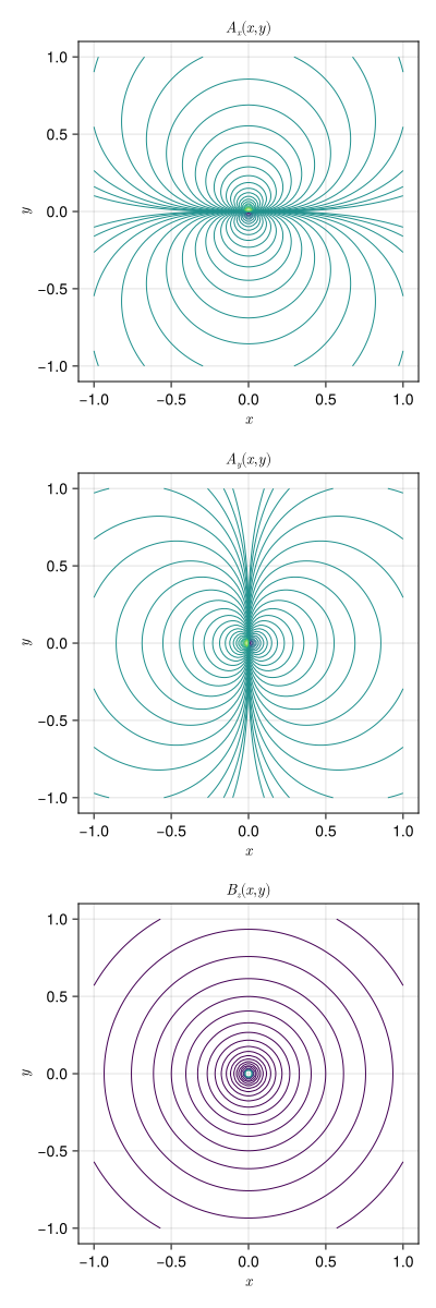
Evaluating the Field
field = FieldFunctions(equ)The divergence is steep enough to be worth keeping in mind when this field is used as a test case — an order of magnitude closer to the axis means three orders of magnitude in $|B|$:
[B(field, 0.0, r, 0.0, 0.0) for r in (1.0, 0.1, 0.01)]3-element Vector{Float64}:
1.0
999.9999999999991
1.0000000000000001e6